01 · INPUT
Raw EVENTS
Historical 2.1.filter MOS1 ori event; SHA-256 has been checked. Extract the raw 1-s broad rate.
Isolated method audit · 2026-09-03
A step-by-step decomposition from event data to trial GTIs, Al/Si sub-spectrum fits, and quartic crossings. The goal is to answer: why does the Al-line scan look discontinuous?
← Return to the original M31 2.1 selection overview
2.1qdp51 time estimator: the 1-s rate enters selection after centered 51-s smoothing. It is not a replacement for the historical 2.1.filter ; no 3B/4.background spectra or response were extracted, and no SP physical judgment was made.
Counting statistics of the Al line are not the dominant problem. The first-scan full spectrum has 21,313 counts in 1–2 keV, with fit χ2/dof=152.7/141=1.08; the low/high sub-spectra near the crossing still have 3,993/17,320 counts, with 1.37 and 1.00, respectively.The second-scan full/low/high spectra likewise have 8,862/4,022/4,840 counts, respectively.
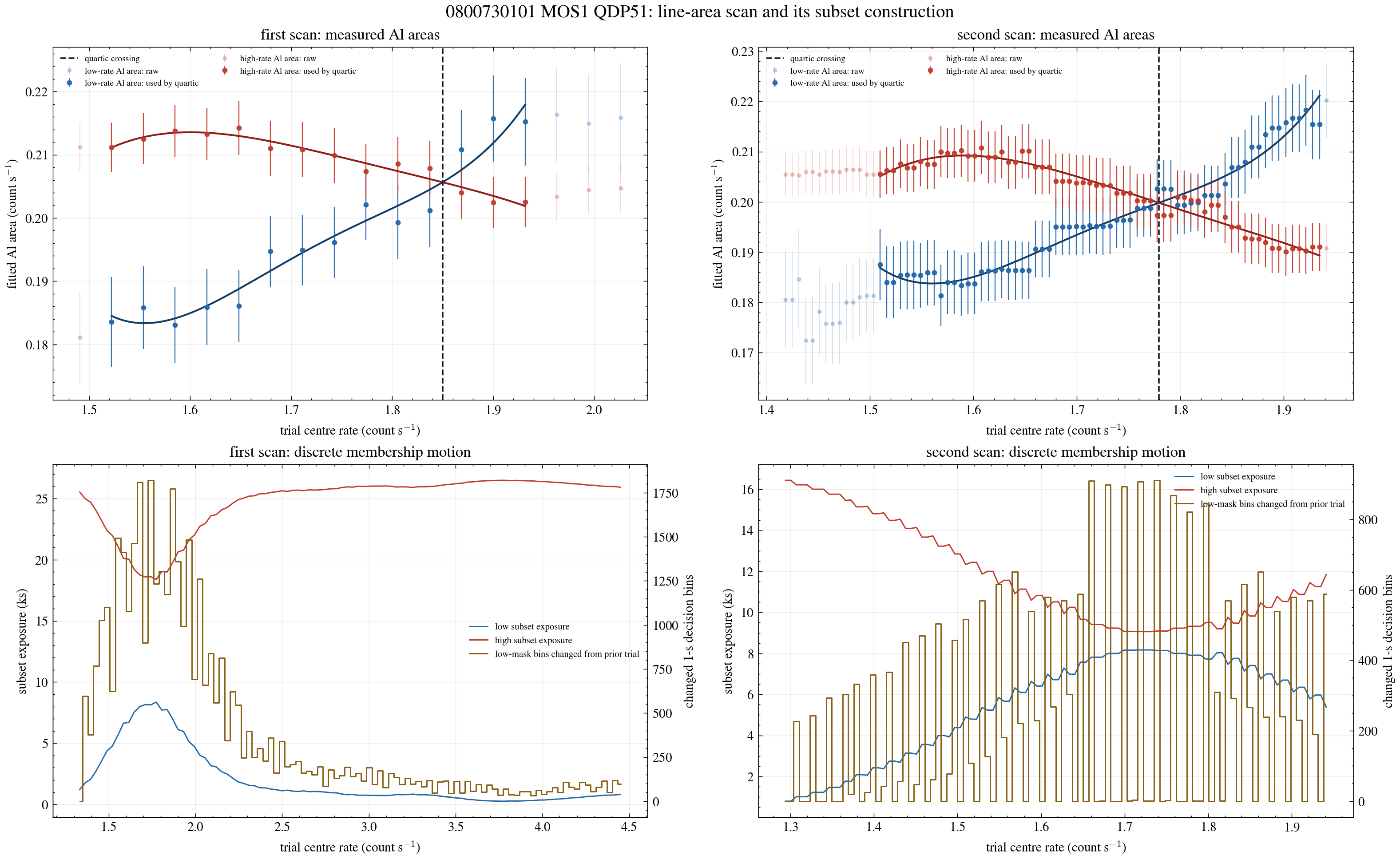
The steps come from sample construction. Each trial centre rate shifts a finite-width rate window to the right. The low subset is not a nested expansion of the previous subset: one set of times is added while another is removed. Thus every fit uses different time intervals, exposure, and grouping; the premise that “line area changes continuously with rate” does not hold.
Below is the actually executed QDP51 branch. Apart from the time estimator, it retains the current 2.1 broad-detector PI=0.2–10 keV definition, two scan rounds, the Poisson σ formula, zero-rate-neighbor rejection, and the BTI guard.
Historical 2.1.filter MOS1 ori event; SHA-256 has been checked. Extract the raw 1-s broad rate.
The decision rate at each 1-s time comes from a local 51-s window; adjacent samples share 50/51 seconds and cannot be treated as independent measurements.
For each m, construct m ± 0.8√(m/51) low/high GTIs. Scan the full interval first, then use subsets within the first-pass GTI for the second round.
Each trial low/high sub-spectrum is grouped independently with ≥100 counts and ≥6 PI channels, then fitted with continuum + Al + Si; the line centroid/width for that round is fixed from the full spectrum.
After removing NaN/MAD outliers, fit 4th-degree polynomials to the low/high Al areas separately; select the root within the scan range and closest to the histogram peak.
The top row shows the Al area and error bar obtained for each trial; pale points are the raw scan, and solid points are those entering the quartic after outlier filtering. The bottom row is not a fit result: it shows how each trial reconstructs the subset. Blue/red indicate low/high exposure, and brown indicates 1-s decision bins whose membership changed relative to the previous trial.
high exposure / low exposure ≤ 6; the actual ratio spans 2.20–99.19.There is no evidence of “complete fit failure”. Columns are full, low, and high; each upper panel shows data, the total model, continuum, Al, and Si components, while the lower panel retains normalized residuals and vertical error bars. Note: this is a detector-space screening model internal to the filter, not a response-folded astrophysical spectral fit.
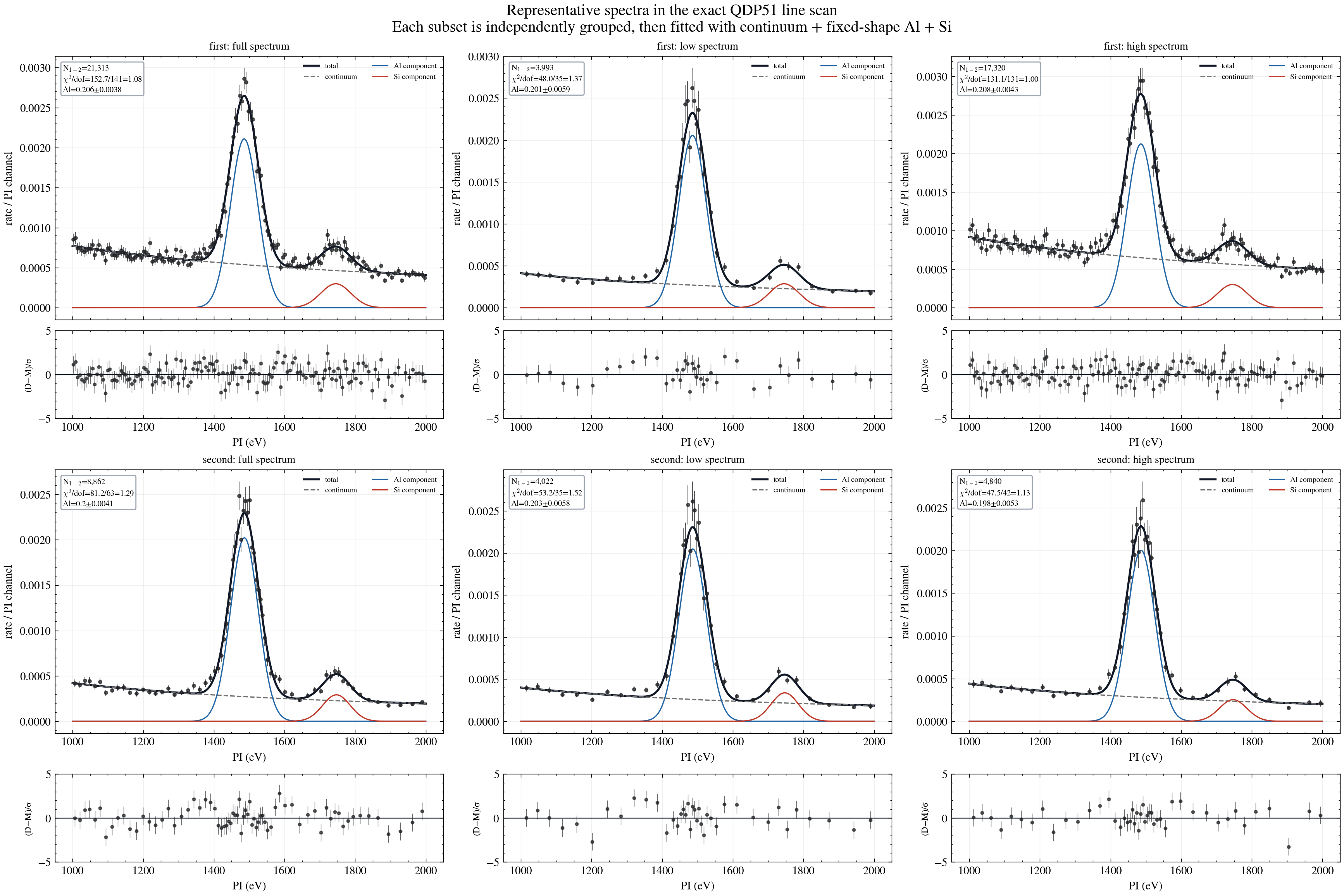
| stage / subset | 1–2 keV counts | grouped bins | χ²/dof | Al area (count/s) |
|---|---|---|---|---|
| first / full | 21,313 | 149 | 152.7 / 141 = 1.08 | 0.2063 ± 0.0038 |
| first / low | 3,993 | 39 | 48.0 / 35 = 1.37 | 0.2012 ± 0.0059 |
| first / high | 17,320 | 135 | 131.1 / 131 = 1.00 | 0.2079 ± 0.0043 |
| second / full | 8,862 | 71 | 81.2 / 63 = 1.29 | 0.2001 ± 0.0041 |
| second / low | 4,022 | 39 | 53.2 / 35 = 1.52 | 0.2026 ± 0.0058 |
| second / high | 4,840 | 46 | 47.5 / 42 = 1.13 | 0.1982 ± 0.0053 |
| Source | Evidence in this case | Meaning for the crossing |
|---|---|---|
| Selection-set jumps | The sliding finite window makes the low/high GTIs non-nested; each step replaces up to 1,820 decision bins, and the GTI is split into hundreds of segments. | Al area is a statistic of a different time mixture and should not be assumed to be a continuous function. |
| Regrouping and joint fitting at every trial | Low/high are grouped independently for every trial, while the continuum and both line areas are free simultaneously; the area of a given line correlates with the continuum slope and the Si line. | The error bars describe a single fit to a fixed subset and do not include systematic uncertainty from subset selection or the crossing. |
| Post-processing interpolation | Only 14 first-scan points and 66 second-scan points enter the degree-4 polynomial; the root is obtained from the difference between the two fitted curves. | Reporting a numerical crossing is not equivalent to measuring a physical transition with an uncertainty. |
The current code sets np.polyfit before w = 1 / area_err**2. However, np.polyfit of w multiplies the unsquared residual directly; for Gaussian errors, the documented convention is w = 1 / sigma. Therefore, points with smaller errors are currently weighted in the objective as 1/σ⁴ rather than 1/σ² , making the quartic crossing more sensitive to a few points.NumPy documentation
This is not a strategy silently modified by this page. This page only exposes it. The next step should separate this weighting correction from “fixed grouping / bootstrap crossing / nested cumulative split” as independent control experiments, rather than changing them together with the GTI policy.
All numbers on the page come from the same diagnostic rerun: event SHA-256 b3851726…e3bfc9, ESPFILT SHA-256 3aad44d2…97ddd. No new GTI, clean event, or background spectrum was written.